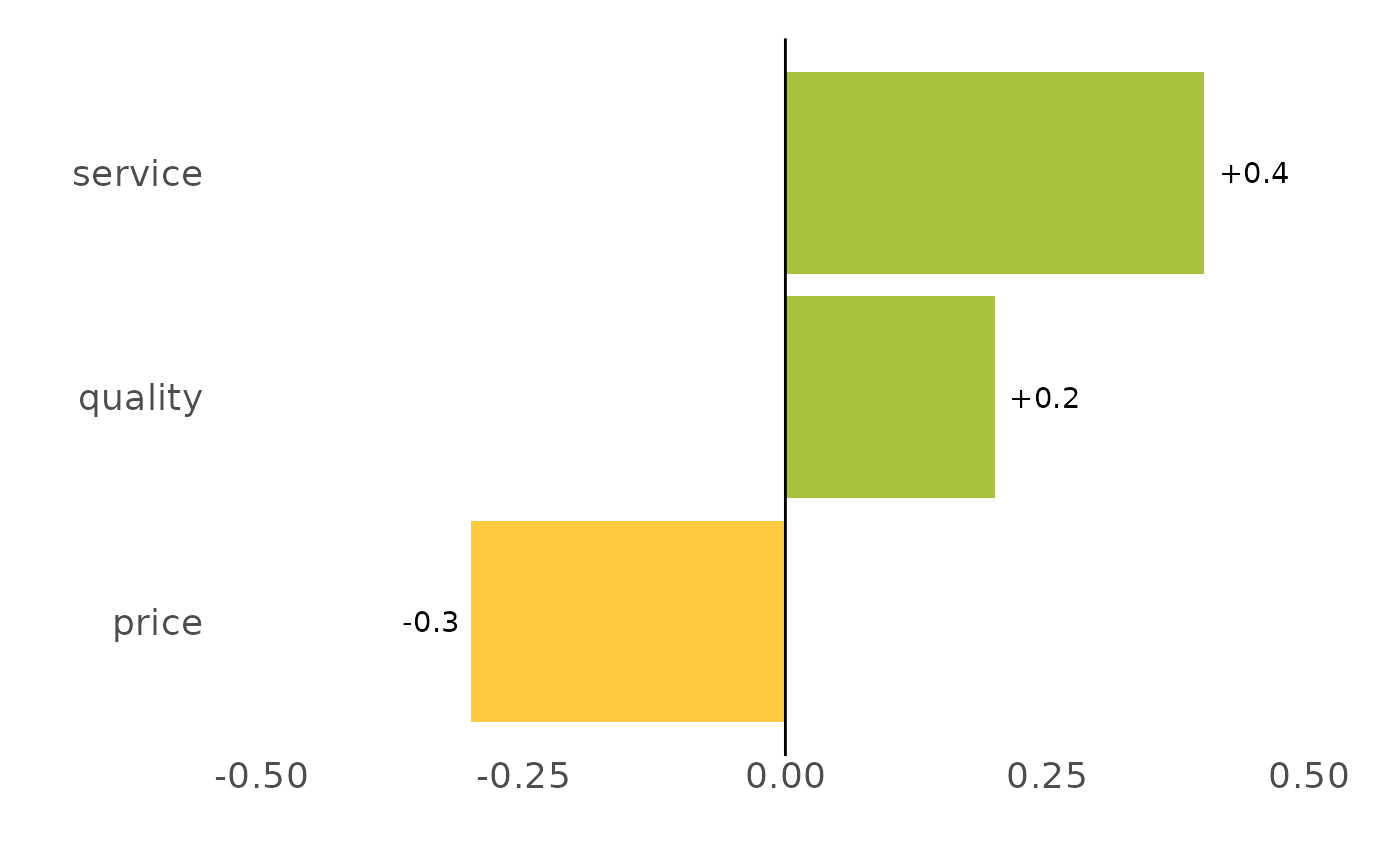
Plots a column of differences (e.g. from compare_values()) as a sorted,
diverging horizontal bar chart: positives in green, negatives in amber, signed
value labels, and a zero reference line. This is the standard "what improved,
what slipped" change chart.
Usage
plot_diff(
  data,
  label = feature,
  difference = difference,
  limits = NULL,
  digits = 2,
  pos_colour = "#A7C23D",
  neg_colour = "#FFCB3E",
  title = NULL
)
Arguments
- data
A data frame with a label column and a difference column.
- label
Category/label column (unquoted). Default
feature.- difference
Difference column (unquoted). Default
difference.- limits
Numeric length-2 y-axis limits. If
NULL(default), a symmetric range around zero is chosen from the data.- digits
Decimal places for the value labels. Default
2.- pos_colour, neg_colour
Bar colours for positive / negative differences.
- title
Optional plot title.
Details
Bars are sorted by the difference and drawn horizontally (largest gain at the
top), coloured green for positive and amber for negative changes, with signed
value labels (+0.20 / -0.30) nudged to sit just outside each bar and a
zero reference line. When limits is NULL the y-axis is made symmetric
around zero from the data so gains and losses are visually comparable; pass
limits = c(-1, 1) (say) to fix it. Feed it the output of compare_values(),
or any data frame with a label column and a numeric difference column.
See also
Other compare:
compare_values()
Examples
a <- data.frame(feature = c("price", "quality", "service"),
                performance = c(3.1, 4.2, 3.5))
b <- data.frame(feature = c("price", "quality", "service"),
                performance = c(2.8, 4.4, 3.9))
compare_values(b, a) %>% plot_diff()