
ezrsurvey turns the things consumer-survey analysts do
over and over into single-line helpers. This vignette walks through a
typical analysis of the bundled podracing_survey dataset:
from raw answers to percentages, models, diagnostics and a chart you
could drop on a slide.
library(ezrsurvey)
#> Loading required package: dplyr
#>
#> Attaching package: 'dplyr'
#> The following objects are masked from 'package:stats':
#>
#>     filter, lag
#> The following objects are masked from 'package:base':
#>
#>     intersect, setdiff, setequal, union
#> Loading required package: ggplot2
#> Loading required package: tidyr
#> Loading required package: tibble
#> Loading required package: readr
#> Loading required package: stringr
#> Loading required package: purrr
The data
podracing_survey is 1,000 simulated respondents with
demographics, a 0–10 NPS question, worded feature ratings, multi-select
motivations, brand questions and open-text comments.
podracing_survey[, c("respondent_id", "demo_gender", "demo_age", "nps_value")]
#> # A tibble: 1,000 × 4
#>    respondent_id demo_gender demo_age nps_value
#>    <chr>         <chr>          <int>     <int>
#>  1 R00001        Male              35        10
#>  2 R00002        Male              29         6
#>  3 R00003        Male              16        10
#>  4 R00004        Male              16        10
#>  5 R00005        Male              16         9
#>  6 R00006        Male              36         9
#>  7 R00007        Male              30        10
#>  8 R00008        Female            23         9
#>  9 R00009        Female            23        10
#> 10 R00010        Male              39         9
#> # ℹ 990 more rows
Percentages without the
count/mutate/pivot_wider
dance
calc_percentage() is the workhorse: counts, percentages
and ordering in one call.
calc_percentage(podracing_survey, demo_gender, sort = "desc")
#> # A tibble: 3 × 3
#>   demo_gender     n   pct
#>   <fct>       <int> <dbl>
#> 1 Male          525    55
#> 2 Female        399    42
#> 3 Non-binary     27     3
Group with by, and pivot to a wide cross-tab with
wide = TRUE:
calc_percentage(podracing_survey, satis_return, by = region, wide = TRUE)
#> # A tibble: 5 × 6
#>   region        Likely `Not sure` Unlikely `Very likely` `Very unlikely`
#>   <chr>          <dbl>      <dbl>    <dbl>         <dbl>           <dbl>
#> 1 Asia              24         25       12            34               5
#> 2 Europe            28         25       16            25               6
#> 3 Latin America     30         21       11            28              10
#> 4 North America     26         24       17            24               8
#> 5 Oceania           31         12       24            24              10
Check-all-that-apply questions live in a block of columns sharing a
prefix; calc_percentage_multi() handles the per-respondent
denominator for you:
calc_percentage_multi(podracing_survey, "motivations_",
                      id = respondent_id, sort = "desc")
#> # A tibble: 5 × 3
#>   option        n   pct
#>   <fct>     <int> <dbl>
#> 1 speed       772    79
#> 2 drivers     533    54
#> 3 social      437    45
#> 4 tradition   349    36
#> 5 betting     295    30
Spreadsheet exports, Google Forms among them, instead pack every answer a respondent ticked into a single cell. The same function recognises that shape and separates the answers, so you do not have to reshape anything first:
packed <- data.frame(
  respondent = 1:4,
  motivations = c("Speed; Drivers", "Speed", "", "Betting; Speed")
)

calc_percentage_multi(packed, "motivations", id = respondent, sort = "desc")
#> # A tibble: 3 × 3
#>   option      n   pct
#>   <fct>   <int> <dbl>
#> 1 Speed       3   100
#> 2 Betting     1    33
#> 3 Drivers     1    33
Note the denominator: three respondents ticked something, so “Speed”
is 3 of 3. When you need those answers as columns rather than as a
table, for a crosstab or a filter, split_multi() widens
them:
split_multi(packed, motivations)
#> # A tibble: 4 × 5
#>   respondent motivations      motivations_Speed motivations_Betting
#>        <int> <chr>            <chr>             <chr>
#> 1          1 "Speed; Drivers" "Speed"           ""
#> 2          2 "Speed"          "Speed"           ""
#> 3          3 ""               ""                ""
#> 4          4 "Betting; Speed" "Speed"           "Betting"
#> # ℹ 1 more variable: motivations_Drivers <chr>
Reusable level orders
Rather than retyping levels = c(...), register an order
once and link it to a variable; calc_percentage() then
applies it automatically.
register_order(
  "education",
  levels = c("Primary or less", "Lower secondary", "Upper secondary",
             "Short-cycle tertiary", "Bachelor or equivalent",
             "Master or equivalent", "Doctoral or equivalent"),
  vars = "demo_edu"
)

calc_percentage(podracing_survey, demo_edu)
#> # A tibble: 7 × 3
#>   demo_edu                   n   pct
#>   <ord>                  <int> <dbl>
#> 1 Primary or less           42     4
#> 2 Lower secondary          111    11
#> 3 Upper secondary          295    30
#> 4 Short-cycle tertiary     123    13
#> 5 Bachelor or equivalent   244    25
#> 6 Master or equivalent     122    13
#> 7 Doctoral or equivalent    35     4
Net Promoter Score
calc_nps(podracing_survey, nps_value)
#> # A tibble: 1 × 8
#>       n   nps pct_detractors pct_passives pct_promoters detractors passives
#>   <int> <dbl>          <dbl>        <dbl>         <dbl>      <int>    <int>
#> 1  1000     7             25           43            32        252      426
#> # ℹ 1 more variable: promoters <int>
plot_nps(podracing_survey, nps_value)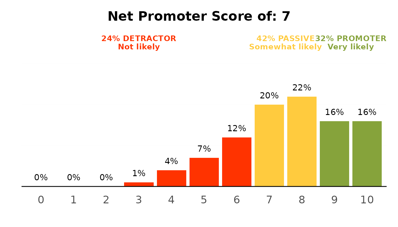
Importance / performance
ipm_model() combines driver importance (by default,
relative weights against the NPS score) with feature performance;
plot_ipm() draws the matrix. Pass
method = "forest" for a random-forest cross-check, which
sees non-linear effects that relative weights cannot.
model <- ipm_model(podracing_survey, nps_value, "ratings_")
#> Parsing `nps_value` as a non-binary variable.
#> Applying multiple regression to calculate relative weights...
model
#> # A tibble: 6 × 4
#>   feature    importance performance perf_class
#>   <chr>           <dbl>       <dbl> <fct>
#> 1 value           24.9         2.86 2
#> 2 atmosphere      23.8         3.57 3
#> 3 speed           18.0         3.48 3
#> 4 safety          14.1         2.88 2
#> 5 venue           12.2         3.08 3
#> 6 commentary       6.99        2.58 2
Comparing two events
For event surveys you often compare this wave with the last.
compare_values() computes the differences and
plot_diff() draws the change chart.
previous <- transform(model, performance = performance - c(.3, -.1, .2, 0, .1))
#> Warning in performance - c(0.3, -0.1, 0.2, 0, 0.1): longer object length is not
#> a multiple of shorter object length
compare_values(model, previous) %>%
  plot_diff()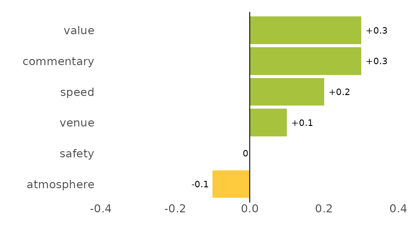
How precise is it?
diagnose() reports the standard error, relative standard
error and margin of error for any column – numeric (point) or
categorical (proportion).
diagnose(podracing_survey, demo_gender, nps_value)
#> # A tibble: 2 × 9
#>   variable    type  unit       n estimate    se   rse   moe precision
#>   <chr>       <chr> <chr>  <int>    <dbl> <dbl> <dbl> <dbl> <chr>
#> 1 demo_gender prop  ppt      951    55.2   1.61  2.92  3.16 high precision
#> 2 nps_value   mean  points  1000     7.56  0.06  0.74  0.11 high precision
For a one-shot, plain-language read on the whole study,
precision_summary() picks the point-scale and proportion
variables for you and writes the bullet points you would otherwise
hand-craft for a report appendix:
precision_summary(podracing_survey)
#> Survey precision summary
#> - Based on 1,000 total responses (per-question base of 776 to 1,000).
#> - Point ratings carry a sampling margin of about +/-0.40 points (up to +/-0.69) at 95% confidence.
#> - Percentages carry a sampling margin of about +/-3.0 percentage points (worst case +/-3.1 at a 50/50 split).
#> - Overall relative standard error of about 4.2% -- high precision.
Why relative standard error?
A standard error on its own is hard to judge – is ±0.05
good? It depends on the scale. The relative standard
error (RSE) divides the standard error by the estimate, so
precision becomes comparable across a 1–5 rating and a percentage alike.
Rating estimates by their RSE is the approach national statistical
agencies use to decide whether a number is solid enough to publish. The
Australian
Bureau of Statistics, for example, treats an RSE of 25% or more as
not reliable for most purposes, marks estimates between 25% and 50% with
an asterisk as ones to use with caution, and suppresses anything above
50%. ezrsurvey keeps that 25% boundary and adds tighter bands below it,
because in consumer-survey work the question is usually which of several
adequately precise numbers to lead with:
| RSE | Rating |
|---|---|
| under 5% | high precision |
| under 10% | precise |
| under 15% | satisfactory |
| under 25% | use with caution |
| 25% or more | likely reliability issues |
For proportions, the margin of error is widest at a 50/50 split
(sqrt(0.5 * 0.5 / n)), so a single worst-case
± percentage-point figure at your achieved sample size
bounds every percentage in the study – which is why
precision_summary() reports it.
Saving and exporting
Every table and plot has a one-line, pipe-friendly save. A bare file
name lands in an ezrsurvey-outputs/ folder, created on
demand, so a script’s results collect in one place instead of scattering
through the working directory; pass a path with a directory in it
("./gender.xlsx", "tables/gender.xlsx",
anything absolute) to put a file exactly where you want it. The first
save of a session says which folder it used, so nothing goes
missing.
calc_percentage(podracing_survey, demo_gender) %>% save_data("gender.xlsx")
plot_nps(podracing_survey, nps_value) %>% save_plot("nps.png")

# several tables, one tab each
export_xlsx(
  gender = calc_percentage(podracing_survey, demo_gender),
  job    = calc_percentage(podracing_survey, demo_job),
  path   = "summary.xlsx"
)
Where to next
- Set persistent defaults with
ezrsurvey_options()and a profile (use_ezrsurvey_profile()). - Build a deck with
report_deck()or scaffold a Quarto report withscaffold_report(), which drops the.qmdbeside where its render will land. - Draft the narrative around the tables with the companion
ezrintelligencepackage.