Stacked score gauges (NPS over average quality, etc.)

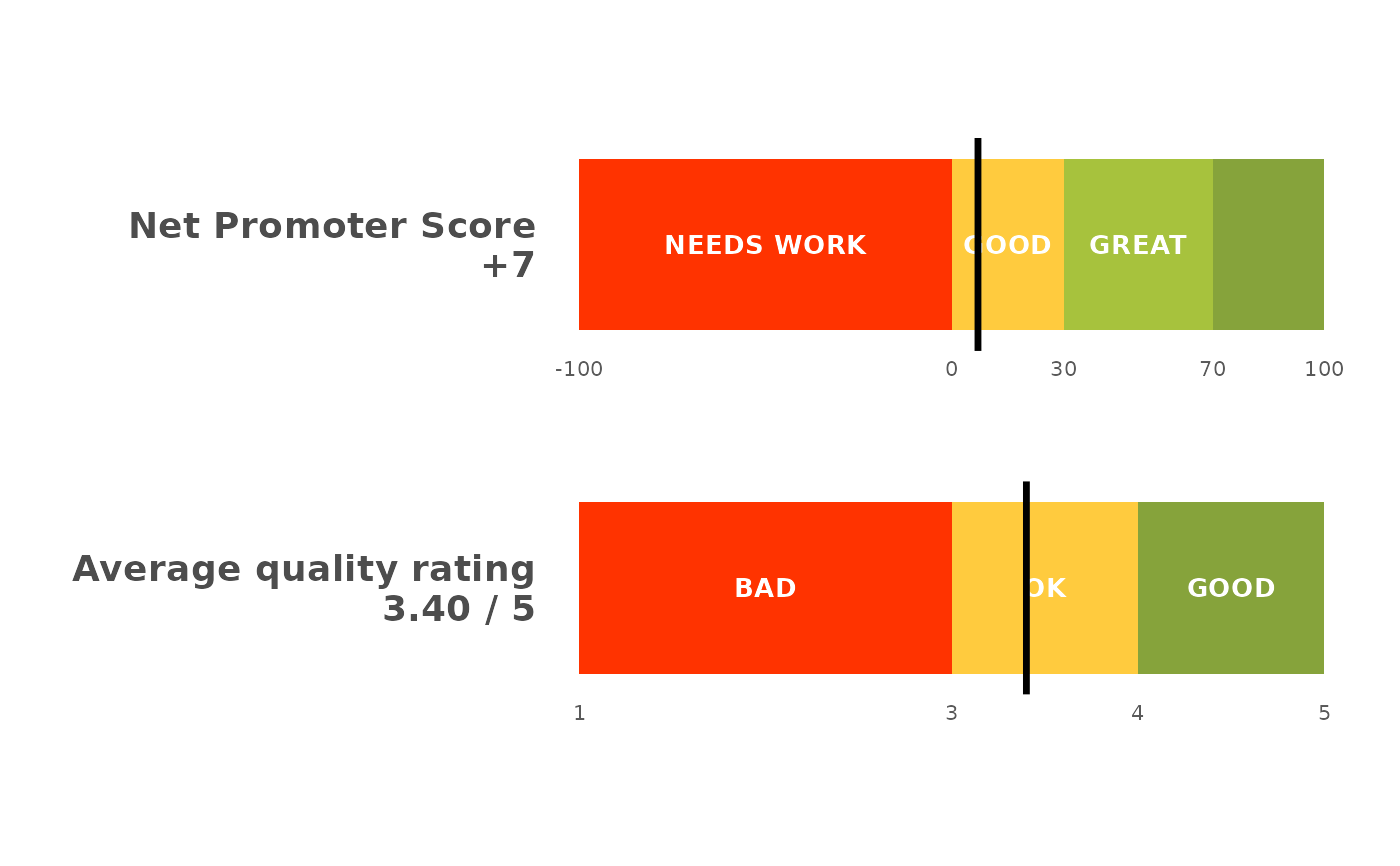
Draws two or more scores as thin banded gauge bars stacked one above another, each on its own scale with a "you are here" marker. The headline summary slide: the Net Promoter Score on top and the average feature quality rating below it, so both key numbers sit together instead of one fat bar filling the slide.

Usage

plot_gauges(
  scores,
  scales = NULL,
  title = NULL,
  height = 0.5,
  label_size = NULL
)

Arguments

scores

A named numeric vector; each name labels a gauge and each value is placed on its scale. The first is drawn at the top.

scales

Which band scale each gauge uses: "nps" (a -100..100 Net Promoter scale) or "rating" (a 1..5 quality scale). Length 1 (recycled) or one per score. NULL (default) infers "rating" for a value in 1..5 and "nps" otherwise.

title

Optional title. NULL (default) draws none, so a slide title can carry the wording instead.

height

Bar thickness in plot units (row spacing is 1). Defaults to 0.5, keeping each bar deliberately thin so several share the panel.

label_size

Band-label text size. NULL (default) is a compact 10 / .pt.

Value

A ggplot object.

Details

Each gauge is normalised to its own scale, so an NPS of +23 and a quality rating of 3.4 line up on a shared 0..1 panel with the band boundaries drawn where each scale puts them (the NPS gauge reuses the plot_nps_gauge() bands; the rating gauge uses bands_rating_3()). The score for each gauge is printed beside its label, and a black marker shows where it lands. Because the bars are thin and stacked, this is the summary-slide companion to the detailed plot_nps() distribution and the plot_ipm() driver matrix.

Since the bars share one panel but not one scale, no axis can serve them both. Each bar therefore carries its own band boundaries as small numbers underneath, so an NPS bar reads -100 0 30 70 100 and a rating bar reads 1 3 4 5; without them a marker two thirds along says nothing about the score it marks. A band too narrow to hold its name is left unlabelled rather than having the text run over its neighbours, and those numbers are what still place it.

See also

plot_nps_gauge(), calc_nps(), ipm_model().

Other plots: plot_bars(), plot_ipm(), plot_nps(), plot_nps_gauge(), plot_quotes_tree(), plot_rating_grid(), plot_stacked_rating()

Examples

nps <- calc_nps(podracing_survey, nps_value)$nps
quality <- 3.4
plot_gauges(c("Net Promoter Score" = nps,
              "Average quality rating" = quality))